Relative error ellipses show the horizontal positional random error between two points, which is what’s tested in some important accuracy standards for property boundary surveys, such as the Minimum Standard Detail Requirements for ALTA/NSPS Land Title Surveys, and Wis. Admin. Code A-E 7.06. The ellipses are incredibly flexible, able to describe error between points connected by any combination of measurements. The underlying math is complicated though, so there’s some confusion and disagreement about how to meet such standards. The goal of this article is to explain what relative error ellipses are, and aren’t, particularly at the 95% confidence level typically used in standards. Things are simplified here to keep it brief and focus on interpreting adjustment results, but some basic knowledge of random error and least squares adjustments is presumed.
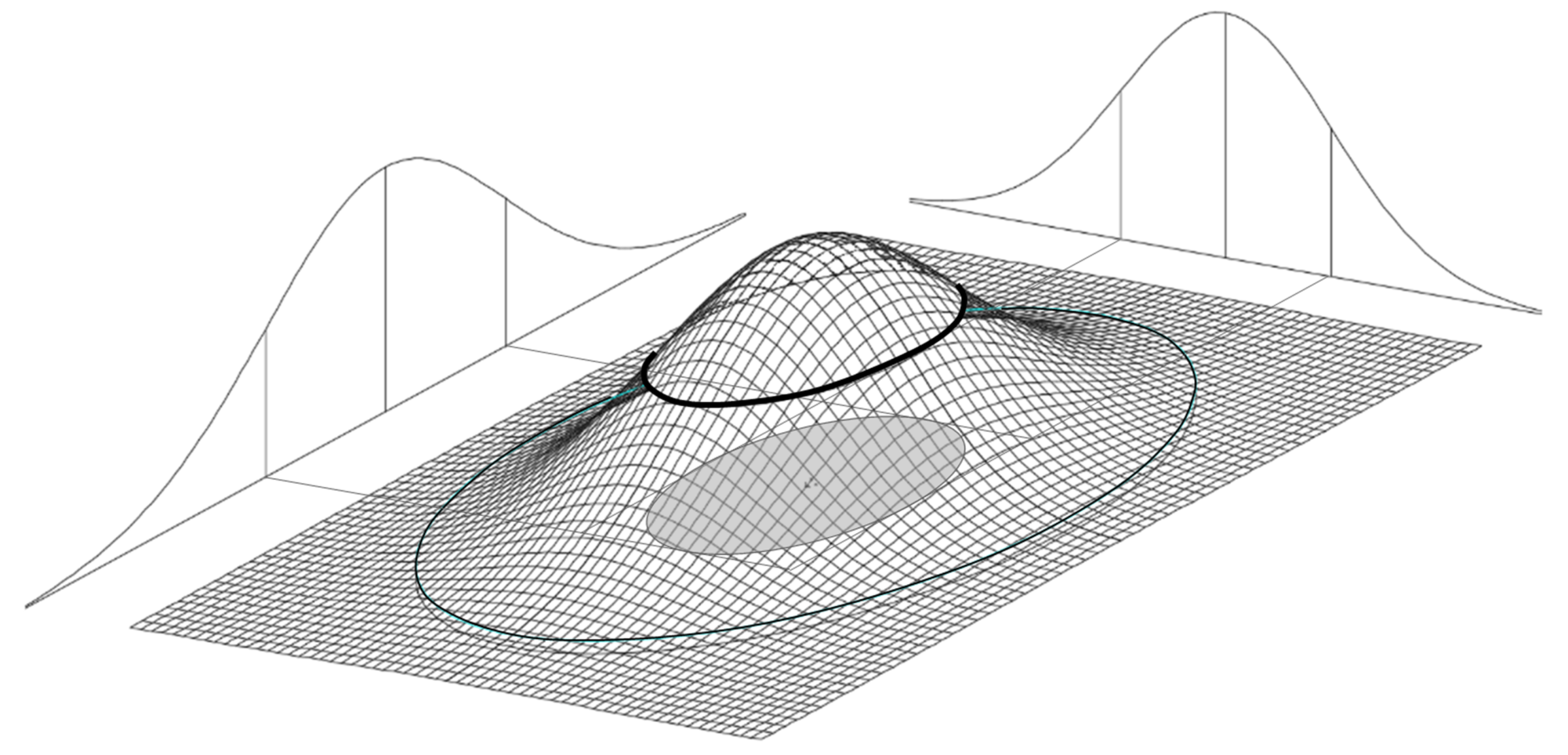
Figure 1: Error Ellipse as Contour Line
What relative error ellipses are:
1.1. Graphically, an error ellipse shows two-dimensional uncertainty due to random error. The true value is probably inside the ellipse (at some percent confidence), and most probably at its center. The ellipse is a contour line of equal probability on a normal distribution (bell-curved) surface.
The normal distribution surface is more complicated than the normal distribution curve that we use for one-dimensional variables (like a single coordinate, distance, or angle), so some things are different, particularly the 95% confidence multiplier (Section 1.8).
1.2. Relative error ellipses are different than point error ellipses. A point error ellipse describes one point’s uncertainty relative to fixed points. A relative error ellipse describes uncertainty of one point relative to another point (uncertainty of the line’s coordinate differences, or its distance and azimuth).
1.3. Mathematically, error ellipses are computed from the variance-covariance matrix, which usually comes from a least squares adjustment. That matrix says how much random error each point’s X or Y coordinate has, and also how each coordinate’s error is correlated (has covariance) with every other coordinate’s error. A point error ellipse is computed from one point’s 3 matrix terms: X and Y error (variance); and XY covariance. A relative error ellipse is computed from two points’ matrix terms, which involves 4 coordinates, so 4+3+2+1 = 10 pairs of error combinations, so 10 matrix terms. The math is complicated, but the number of matrix terms involved shows how a relative error ellipse is more complicated than the point error ellipses on both ends.
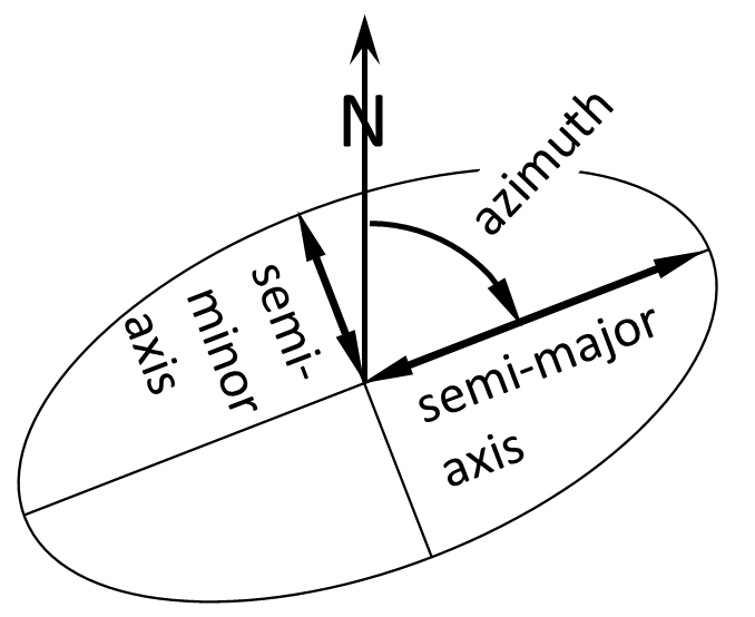
Figure 2: Ellipse Dimensions
1.4. Error ellipses (point and relative) are ultimately described by 3 parameters: the semi-major axis (the “big radius”) and semi-minor axis (the “small radius”) describe the size; and the azimuth of the semi-major axis describes the orientation. Ellipses are also scaled a couple times (Section 1.7 & 1.8). We use the “semi” dimension (like a radius) rather than the total width (like a diameter), because we care about how far the true value could be from our most probable value (ellipse center), not what the total range of true values could be.
1.5. For both point and relative error ellipses, their relative sizes (each ellipse compared to all others in the network) are almost completely determined by: 1) the approximate point locations; 2) what measurements tie them together; and 3) the user-estimated standard errors of those measurements (which weight the adjustment). The actual measured values of course affect the exact point coordinates, and the measurement residuals (how much each actual measurement changed to agree with the others) affect the overall size of all ellipses, but only overall. This is why it’s so important to be honest about the user-estimated standard errors, including instrument and target centering.
1.6. Based on the above, it’s possible to compute error ellipses without any adjustment at all. Some apps (such as Microsurvey StarNet) can generate them without any redundant measurements (just side shots, or an open traverse). Most apps require some redundant measurements, but not necessarily to every point. So, the presence of an error ellipse doesn’t mean that a particular point had an independent check.
Point and relative error ellipses, and other computed errors, are usually scaled twice, as described below:
1.7. First, they may be scaled by the adjustment’s standard deviation of unit weight (a.k.a. reference factor, total error factor), which is basically an overall ratio of residuals (how much measurements had to change in the adjustment) divided by user-estimated standard errors (how big you expected those residuals to be). We expect that factor to be around 1. If there’s nothing to adjust, the factor defaults to 1 (no scaling). Many apps scale both up (>1) and down (<1). Some apps (such as Microsurvey StarNet) only scale up, not down, the rationale being that a small factor is just luck, and doesn’t mean the user-estimated standard errors are really too large. Even more complicated, some apps (such as Microsurvey StarNet) only scale up if the factor is “statistically larger” than 1 (per Chi Square test), the rationale being that a factor “slightly” larger than 1 is also just luck, and doesn’t mean the user-estimated standard errors are really too small.
1.8. Second, error ellipses are also scaled up from “standard” size to 95% confidence using a factor of at least 2.45 (rounded). That’s larger than the 1.96 we usually associate with 95% confidence. It’s larger because an error ellipse is two-dimensional, and it must be magnified by 2.45 in order to enclose 95% of the volume under a normal distribution surface. Compare that to one-dimensional variables (a single coordinate, distance or angle), where a 1.96 multiplier encloses 95% of the area under a normal distribution curve. Figure 3 shows how that puts a lot of the 95% ellipse well outside the 95% coordinate error rectangle, which seems strange, but it is what it is. Complicating things further, some apps use even larger 95% multipliers, because they essentially assume that the user-estimated standard errors (for weighting) are just an unreliable, small set of “sample” standard errors, rather than reliable “population” standard errors. The larger multipliers depend on the degrees of freedom (number of redundant measurements) in the adjustment. As degrees of freedom approaches infinity, the multipliers approach 1.96 (1-D) and 2.45 (2-D). Different apps use one assumption or the other, or let you choose. For example, Microsurvey StarNet and Trimble Business Center use the “population” assumption (always 1.96 & 2.45). Carlson SurvCE gives you a choice. Dr. Charles Ghilani’s Adjustment Computations textbook (John Wiley & Sons) has long used the “sample” assumption.
Regarding both types of ellipse scaling, perhaps we’ll all get on the same page in the future, but the differences have existed probably since we started using computers. For now at least, be aware of the different approaches, and the thinking behind them, which boils down to how much you trust the user-estimated standard errors of the measurements.
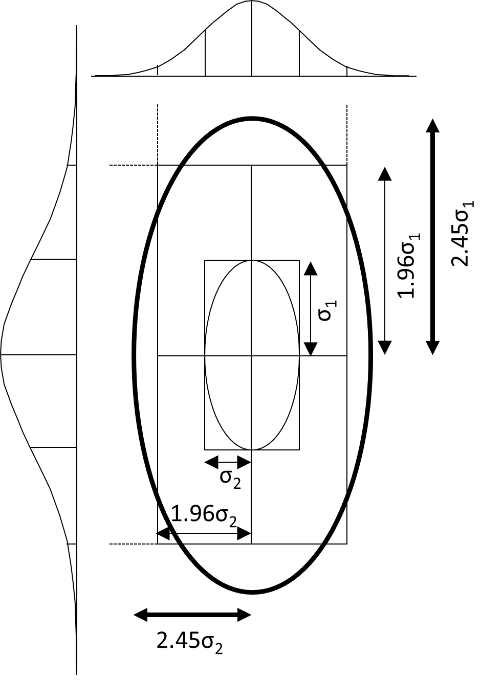
Figure 3: 95% Error Ellipse vs. 95% Coordinate Error Rectangle (simple case – no rotation)
95% scaling check in Excel:
The general 95% multiplier formula in Excel is =SQRT(df1*F.INV(0.95,df1,df2)) df1 = 1 for 1-D variables
df1 = 2 for 2-D variables (ellipses)
df2 = infinite (use 9999999) for the “population” assumption
df2 = network degrees of freedom for the “sample” assumption.
Selected 95% multipliers are listed below. Note how big they get with few degrees of freedom (df2).
df2 1-D (df1=1) 2-D (df1=2)
1 12.7062 19.9750
2 4.3027 6.1644
3 3.1824 4.3708
10 2.2281 2.8645
25 2.0595 2.6020
100 1.9840 2.4849
150 1.9759 2.4724
9999999 1.9600 2.4477
What relative error ellipses are not:
2.1. Relative error ellipses (uncertainty between two points) are not point error ellipses (point uncertainty relative to fixed points).
2.2. Relative error ellipses are not limited to two points directly connected by measurements. They can be computed between any two points in the network. For example, in Figure 5, the points are directly connected with distance and angle measurements, but in Figure 4 they are not. Figures 4 and 5 only show relative error ellipses between adjacent points, but they also exist between more distant points.
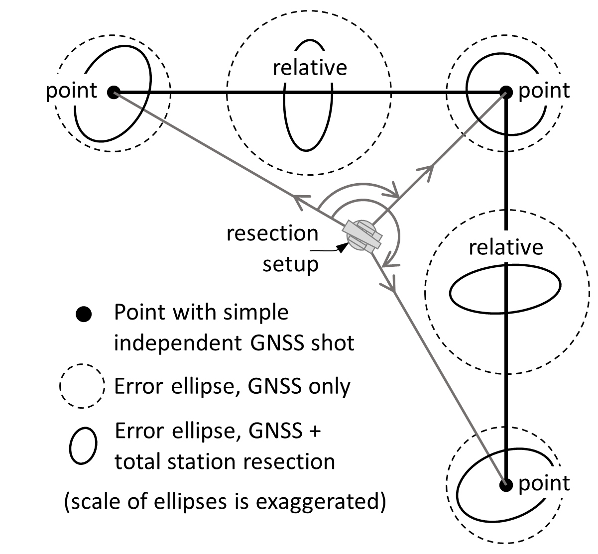
Figure 4: Relative Error Ellipses Can Be Complex
2.3. Relative error ellipses are not necessarily a simple function of the point ellipses on either end. A simple situation in which they are, would be two points shot independently with RTK GNSS (no covariance between points), with each point error ellipse being circular (no more X error than Y error, and no covariance between X and Y error at a point). In such a simple situation, the complicated error propagation simplifies to the “error of a sum” principle, where the relative error ellipse’s (circle’s) radius is the square root of the sum of squares of the radii of each point error circle (dashed circles in Figure 4). In more complicated situations, like when measurements tie points together locally, there can be covariance between points, and/or covariance between one point’s coordinates. So generally, “error of a sum” does not always apply, and the true relative error ellipse must be rigorously calculated from the variance-covariance matrix.
2.4. Relative error ellipses are not quite the same as the computed azimuth and distance errors between points. One issue is orientation — if the ellipse axes aren’t aligned parallel / perpendicular to the line, then the semi-major axis can be larger than both the azimuth error and distance error of the line. How much larger depends on the ellipse shape and orientation. Another issue is scaling to 95% confidence — some apps assume the line’s azimuth and distance errors are separate one-dimensional errors, scaling them to 95% by 1.96 instead of 2.45 (or larger scales per “sample” vs. “population” issue in Section 1.8). Other apps assume the azimuth and distance errors work together to describe two-dimensional error, and therefore scale them by 2.45 like error ellipses are scaled.
2.5. Relative error ellipses are not necessarily independent of which points are held fixed. Consider a pair of points “farther” from (with weaker ties to) fixed points (Figure 5). Obviously, their point error ellipses should be larger. Their relative error ellipse could be larger too, mostly because the direction (azimuth) component of that error is relative to north, not relative to an adjacent line. Even with minimum horizontal constraints of one fixed point and one fixed azimuth, moving those fixes closer to the problem points could shrink both the point and relative error ellipses. This is the sort of change that can “juke the stats” just to meet a standard. The right thing to do is fix what you should fix (probably the GNSS base(s), or section line), and instead improve your network, probably by adding GNSS shots in the problem area.
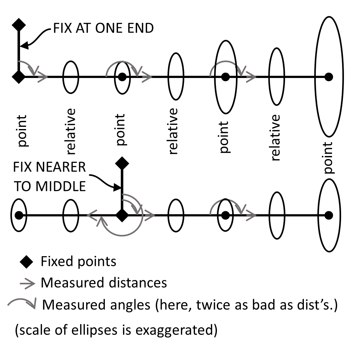
Figure 5: Changing What’s Fixed can Change Relative Error Ellipses
2.6. Small error ellipses (point or relative) do not by themselves guarantee that blunders or systematic errors have been removed, or even that the ellipses really show the amount of random error present. Remember that it’s possible to generate error ellipses for unchecked side shots, and that the relative size of each ellipse compared to all the others is very dependent on the user-estimated standard errors of the measurements.
2.7. Error ellipses (point or relative) are not a good blunder detection tool. Large measurement residuals in one part of the network do not make just the nearby ellipses larger. Instead, the large residuals make the overall standard deviation of unit weight larger, which scales all ellipses. Blunder detection is best done by examining the measurement residuals themselves, understanding that a single blunder tends to cause many large residuals in that part of the network.
Summary:
If you really want to know the 95% uncertainty between any two Points A and B in your survey, do the whole survey 1,000 times, compute 1,000 pairs of (Xa-Xb) and (Ya-Yb) coordinate differences, plot them, and best-fit an ellipse that includes 950 of the 1,000 data points. That’s impractical, so we instead use statistical theories to estimate how such repeated surveys would vary. Least squares and error ellipses are complicated, they depend heavily on user honesty, and different apps scale the final errors differently. However, these tools are universal (mix GNSS, total station and leveling in any network configuration) and also flexible (measure in any order – start topo before finishing control), which is why many modern accuracy standards are based on them. They are also showing up in more of our procedures, such as total station resection setups. They are another modern-age black box that we surveyors may never understand completely, but should still learn enough about to use them competently (particularly the different scale factors for 95% confidence).
Finally, keep least squares and error ellipses in perspective. They alone are no guarantee of a good survey, and lots of good surveys have been done without them. For property boundaries, they can’t tell you whether you’ve done enough research and looked hard enough for the right points to measure to in the first place, nor how to reconcile that field evidence with other evidence in order to locate the boundary. The essential app for that is an experienced surveyor’s professional judgement!
Dan Rodman is a Wisconsin Professional Surveyor & Civil Engineering Technology instructor at Madison College, Madison WI drodman@madisoncollege.edu